7 Ways to conditionally calculate sum of values in Excel.

Excel offers different ways to accomplish the same task. This is especially evident in the case of using Excel functions, where we can simply choose the one that offers the best solution, or more realistically, the one that we are more comfortable using. As an example, let’s solve the following scenario: We are offering online Excel courses both: on our internal website, as well as on Udemy’s platform. Udemy charges us 50% fee on all course sales, and also offers promotional rates to increase our volume. As a result, we are selling the same content at different prices. Looking at Thanksgiving week sales performance, let’s calculate our total Net Sales for all of Udemy transactions (highlighted). Let’s use different Excel functions to perform calculation required.

Method 1 – Use the SUBTOTAL function while filtering your rows
We covered using SUBTOTAL function in our last post. This method has its limitations, as we are required to actually filter our data and cannot perform this calculation on the fly. Otherwise, this could be a route that we can take.
Method 2 – Use the SUMIF function
=SUMIF(range,criteria,[sum range])
This function would allow us to calculate the sum of range specified based on our condition applied to the criteria range. In our example, our criteria range is Web Platform: $C6:$C$22, our condition is the web platform used: “Udemy”, and the range that we would like to be calculated, if match is found is Net Sales: $G$6:$G$22. Our formula becomes the following:
=SUMIF($C$6:$C$22,”Udemy”,$G$6:$G$22)
Method 3 – Use the SUMIFS function
=SUMIFS(sum_range,criteria_range1,criteria1…)
This SUMIFS function, which was introduced in Excel 2007 is enhanced version of the SUMIF function and allows us to perform calculations based on multiple conditions, instead of just one. In our example, let’s adopt it for use with the single condition that we have. There might not be a practical need to use the SUMIFS function for a single criterion sum, however; if needed, we can simply change it to calculate multiple conditions without having to switch functions used. Notice that parameters have a different order in this function, versus the SUMIF function. Our sum_range as was the case before is: $G$6:$G$22. Our criteria_range1 is $C$6:$C$22, and our criterion is “Udemy”. Putting all of the pieces together, we now have:
=SUMIFS($G$6:$G$22,$C$6:$C$22,”Udemy”)
NOTE:All the above examples accept arguments that are ranges(individual cells or ranges of cells ONLY, while the proceeding examples accept arrays as parameters. If a range is given, they simply covert it into an array.
Method 4 – Use the SUMPRODUCT function
=SUMPRODUCT(array1,[array2]…)
Before Excel 2007, SUMPRODUCT was the go-to function for performing multiple-condition sums. The syntax of this function allows us to substitute comma for an asterisk, making this function a bit easier to follow. In our example, we need to “multiply” our Net Revenue by any record found as a match in the Web Platform column for “Udemy”:
=SUMPRODUCT($G$6:$G$22*($C$6:$C$22=”Udemy”))
Method 5 – Use the DSUM function
=DSUM(database, field, criteria)
This under-utilized Excel database function is a little tricky to set up, but very rewarding when dealing with multiple criteria. Our database is the whole range of records, including column headings: $B$5:$G$22. The field parameter accepts either text string of column name, or column’s number in the range. Both: “Net Revenue” and 6 would work for us. Finally, the criteria often requires us to set up some “helper” cells, but in my case, I conviniently use the value from the very first record in our range as my criterion:
=DSUM($B$5:$G$22,6,$C$5:$C$6)
NOTE:The next two functions are array functions, and need to be entered with following keyboard combination: CTRL+SHIFT+ENTER in the formula box. For the Mac users out there, you would have to use COMMAND + RETURN.
Method 6 – Use the SUM function
The syntax is very similar to the SUBOTAL function, but parameters are reversed. We need to specify our condition first, and then “multiply” by the sum range. Don’t forget to use CTRL+SHIFT+ENTER:
=SUM(($C$6:$C$22=”Udemy”)*($G$6:$G$22) )
Method 7 – Use the SUM(IF()) function combination
We simply follow the syntax of the IF function, and perform summation on top of it. Again, you would have to use CTRL+SHIFT+ENTER combination for this formula to work properly:
=SUM(IF($C$6:$C$22=”Udemy”,$G$6:$G$22,0))
Considerations:Using SUMIF, SUMIFS functions would yield much faster speed performance than any other functions used. In addition, using these functions, you can include wildcards in your search criteria. If these functions offer the solution that you need, you should use them. However, you can choose to use other examples provided, when you need to overcome these functions’ limitations: passing array parameters, or using calculations or expressions as search conditions…
Method 8 (BONUS!) – Using PivotTables approach.
PivotTable functionality is another Excel tool we can incorporate into calculalating results required, however they deserve a separate post or a series of articles.

Examples with multiple search conditons:
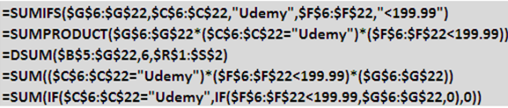
Using SUMIFs function for the single search condition might be an overkill, let’s change our criteria to only include discounted Udemy courses. Feel free to download companion workbook for this post, and find solutions below. Please note creation of R1:S2 “helper” data range to for setting up DSUM function. Also note that the array version of the IF statement does not allow usage of AND function, so I had to take the nested IF function approach. In addition, we cannot use the SUMIF function any longer, since it can only handle one condition at a time:
What are your thoughts on this topic? When it comes to conditional summing of data, which functions do you use and why?
Very usefull information thanks a lot…
I am glad you liked this article, Shafqat! I plan to continue posting more examples to better utilize Excel functions and other program functionalities.
Nothing like knowing multiple ways to solve similar problems, each with their own uses driven by the situation, of course! I definitely use SUMIF and SUMIFS most, following by PivotTables and the SubTotal. DSUM I’ve only used in Access.
I’m not fluent in SUMPRODUCT nor the array formulas, so I use them seldom. That’s probably because my math education ended with Business Calc & Business Statistics. Matrix math hasn’t taken hold in my gray matter. For example, sometimes I see column arguments separated by a comma and sometimes by the multiplication sign. I understand, to some degree, what the formula does in each case but I don’t understand when each is appropriate. IOW, I can read and imitate but writing from scratch would be a challenge.
A couple of months or so ago I ran into a need to average across a row, ignoring hidden columns. Kind of like SubTotal, only sideways. Of course, SubTotal only works when considering hidden rows. I devised a VBA UDF to ignore hidden columns as well as rows, complementing/replacing SubTotal. The process I went through to get to this is on my personal blog (certainly not a competitor to this one!) on a page called “Beyond SubTotal()”.
Thanks for stopping by, Don!
I am a big fan of learning by “imitating” method. It is a much easier, faster way to learn than starting from scratch.
Thanks for pointing out the value of using VBA to fill in some of the gaps in Excel. While Microsoft has enhanced SUBTOTAL function with the introduction of AGGREGATE function in Excel 2010, both of these functions still cannot handle hidden columns.
Anyone who is interested in learning your solution, can follow this direct link:
http://bigdon-in-vbaland.blogspot.com/p/beyond-subtotal.html
GET PROFESSIONALLY VIDEOS AT AFFORDABLE PRICES
We offer professionally produced videos at affordable prices.
Our videos have the look and feel of a high quality television commercial, complete with professional spokesperson, background, text,
images, logos, music and of course, most importantly, your company’s contact information for your excelstrategiesllc.com.
If you’re ready to reach more clients today, let us get to work on producing your company’s exclusive video.
MORE INFO=> http://qejn39630.bloggerbags.com/8235120/get-videos-at-affordable-prices