Solving ModelOff Data Analysis problem from the second round of 2013 competition.

         As some of you might know, Model Off 2014, championship kicked off last Saturday, October 25th. With the first round of this modeling competition behind us, I thought that this might be a good time to tackle one of their older problems. I might be biased here, but starting with their Data Analysis problem made a perfect sense to me. Luckily enough, this could arguably be one of the easiest problems they have ever presented. You can download both: Questions/Answers worksheet and Excel workbook with source data for this problem directly from their website.

         As usual, I will not pretend to have the best possible, optimal solution, I simply offer one which works. Since in the real world, we are not constrained by challenging time restrictions, imposed on ModelOff contestants, I was not concerned about the most efficient solution, but rather the one that is more presentable. As an example, my solution heavily relies on Top Ten filtering feature available for PivotTables, this might seem like an extra step comparing to simply presenting all records and then sorting them in order of preference. In my humble opinion this is a better way to present top 1/3/5/n results, rather than looking at extra records of data.

         My approach to this problem was rather simple: I followed ModelOff’s recommendations of adding some “missing” columns with required calculations to the data source, and then created some PivotTables to answer questions at hand. I thought that we needed to add following columns to the data source: Total Sales, Total Cost, Total Profit, Total Discount, Month, and Invoice Flag:

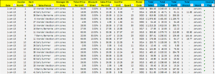
         Since our data source only includes Sales Price Per Unit, and Quantity fields, to calculate our Total Sales, we simple need to multiply them: Total Sales = Sales Price Per Unit * Quantity, or L2=$H2*$J2 . Building on this logic, we have:
         Total Cost = Cost Per Unit * Quantity, or M2=$I2*$J2
         Total Profit = Total Sales – Total Cost, or N2=$L2-$M2
         Total Discount = (Ticket Price Per Unit – Sales Price Per Unit) * Quantity, or O2=($F2-$H2)*$J2

         To quickly answer questions asking us to filter data by Month value, we need to extract it for each date presented. Using MONTH function, we could get a numeric equivalent for each month in the range (1 = January, 2 = February, 3 = March, etc.) However, experimenting with different formatting options for Excel’s TEXT function, we can actually determine month name based on each date in the data source:
         P2=TEXT($A2,”mmmm”) yields January, as A2 happens to be 1/1/2013.

         To complete the setup for our data analysis, we now need to flag UNIQUE occurrences for our Invoice numbers. It’s a shame, but to the best of my knowledge, PivotTables don’t allows to perform unique value counts, and below is just one of many work-arounds we can implement:
         We can create a mixed reference data range for our invoice numbers, and each time total count of invoice number occurrences is 1 (first iteration), we will assign a value of 1 to this field, otherwise (count of occurrences <>1), we will flag it as 0. In other words, all of the consecutive occurrences of the invoice number will be flagged as 0. This strategy allows to accurately count number of unique invoices: Q2=IF(COUNTIF($B$2:$B2,$B2)=1,1,0)

         By now we have all of the data that we need to answer questions for this problem. We just need to create our PivotTables and apply filters to meet criteria used.

         Let’s walk through solution for the first question asked:

         To answer question asked, we will create a new PivotTable : Insert – Pivot Table:

         make sure that we selected all data within our data range:

         and filter the results by placing Item Code field into the Report Filter section and selecting for item code 10, then placing Manager On Duty field into Report Filter and selecting John Jones value, and finishing the problem by placing the Quantity field into Values area:

         You will now see a Pivot Table similar to below (sans formatting options):

         We can now see that 554 is the closest value to 600, and select answer B as our final answer.

         Using the same approach, we can solve the remaining 15 questions of this problem. You are welcome to use my workbook, for additional assistance.