Working with MS Excel Array Functions (FILTER, RANDARRAY, SEQUENCE, UNIQUE, SORT, SORTBY)
It’s hard to keep up with seemingly non-stop additions to Excel’s impressive catalog of functions. If you happen to belong to Office Beta channel you might have started working with the newest release of text and array functions. As a regular Office 365 subscriber I’ve already covered newish XLOOKUP and LAMBDA functions on this blog. It was last year when the Excel team introduced dynamic array functions, also known as spilled array functions. These functions return arrays of of values of different sizes and spill them into adjacent cells. You can usually specify how long and how wide the output ranges should be. These functions include – UNIQUE (returns unique values from the range of values), SEQUENCE (retrieves a sequence of values), SORT, SORTBY, RANDARRAY(array of random numbers based on specified parameters), and FILTER. In this post we will explore examples on how to use these functions.
SEQUENCE Function
This function has four arguments [Rows, Columns, Start, and Step], only the Rows one is required, others are optional.

Suppose we want to create a sequence of numbers by day for sample deposits across twelve bank accounts. We would set up a SEQUENCE function with a value of 12 for Rows and 7 for Columns: =SEQUENCE(12,7), should we go with default values of 1 for both start and step, our output range would be populated by values starting at 1 and ending at 84. Note that this result is equivalent to filling in the formula fully =SEQUENCE(12,7,1,1)
Another example could be populating bank accounts from 100001 to 1000012. Our formula becomes =SEQUENCE(12,1,100001,1), in which we specify that we want to fill 12 columns, 1 row with values starting at 100001 and gradually increasing by 1.
Lastly, should we like to populate days of week starting with Monday and going through Sunday, we can achieve this by combining the SEQUNCE function with the TEXT function via =TEXT(SEQUENCE(1,7,2,1,”DDDD”) formula. As a reminder: Excel considers Sunday to be the first day of the week, hence Monday has a value of 2.
UNIQUE Function
Admittedly I date myself yet again, but when I first started using Excel the only productive way to de-dup values was running your array through a PivotTable. It was not until Data Tools ribbon introduced much anticipated Remove Duplicates button did it become easier for folks to get rid of duplicated values in their data. Having the ability to do anything via a function is always preferable to using an interface and the UNIQUE function only calls for one required argument – Array, leaving remaining two: By_col and Excactly_once optional. The dialog below helps us create unique list of states in our data.

Note that we can de-dup more than one column, given we have values for City in column D and State in column, C; unique list for City/State combinations can be derived via this formula, which will yield 28 values based on the input of 52 possibilities
=UNIQUE($D$6:$D$57&", "&$E$6:$E$57)RANDARRAY Function
If your job requires working with sample data you probably used Excel’s RANDBETWEEN function at some point. With the introduction of RANDARRAY we are able to not only type a formula once and create an array of data, we also have more control over the dummy data we are fabricating: [Rows] argument specifies the number of rows in the desired array, while [Columns] does the same for… columns in your table. [Min] and [Max] are fairly self-explanatory, not unlike RANDBETWEEN’s [Bottom] and [Top] arguments. [Integer] will help specify data type between an integer vs. decimal value. Below example creates a 12×12 matrix with integer values ranging from 100 to 200. Note that the header row is composed using the SEQUENCE function.

=RANDARRAY(12,12,100,200,1)
=SEQUENCE(1,12,2010,1)
SORT Function
In a similar light of relying on Excel formulas vs. GUI to perform basic functionality, the SORT function is a much welcomed addition to the function library. The array is the only required argument here, which asks us to define data range for us to sort. While the default is set to 1, the sort_index argument identifies column number/index in our range. Sorting order is defaulted to ascending, (value of 1), and can be changed via sort_order. Lastly, this function sorts by column, but you can change this preference to row, via the by_col argument.
We can choose to order our list of City/States from the UNIQUE function example above by wrapping UNIQUE function within the SORT function like so
=SORT(UNIQUE($D$6:$D$57&", "&$E$6:$E$57),)
SORTBY Function
Not to be confused with the SORT Funciton, the SORTBY function offers additional flexibility for all of your sorting needs. In fact, it allows us to sort contents of one data range based on the values from a different data range. As such, this function calls for two required arguments. First we need to specify the array to sort – array, then we define the array to sort by – by_array. Optionally, we can define our sorting order (with the default of ascending) via sort_order and order pairs: array/order. Putting both UNIQUE and SORT functions to a good use perhaps we could construct deduped list of colleges, cities and states, conveniently turning our dataset into a table format prior to this manipulation:
=UNIQUE(SORTBY(tblColleges, tblColleges[State],1,tblColleges[City],1),,)
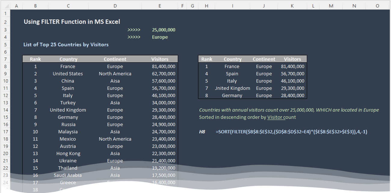
FILTER Function
The next logical interface functionality to replicate after the sort is FILTERing. This function includes two required and one optional arguments. First we need to specify the data range we need to filter – Array. Then we cold define single condition OR multiple criteria to filter our data for – Include. Optionally we can handle errors using If_empty argument. To illustrate let’s work the list of top 25 countries by number of visitors. This table includes Rank, Country, Continent, and Number of annual Visitors. We also added a couple of additional filters/input cells for us to filter this dataset further.

Should we want to list countries with annual visitor count over 25 Million, listed in ascending order by country name, our formula can take this shape:
=SORT(FILTER($C$8:$F3$2,$F$8:$F$32>$F$3),2,)If we need to further limit our list to countries located within Europe AND sort this list in descending order by Visitors, we can do the following:
=SORT(FILTER($C$8:$F$32,($E$8:$E$32=$F$5)*($F$8:$F$32>$F$3)),4,-1)All of the examples listed can be found via Excel file download for this page.
Do you find any of these functions more useful than others?
I’m in the mood for something sweet and spicy… you? – https://rb.gy/es66fc?Fece