Running Statistical Data Analysis (EDA) using Excel Functions and Formulas.

Back in August Microsoft made a momentous announcement of good ole’ Excel now supporting Python scripts (at least for those Office 365 subscribers who are part of the Beta Insider channel.) While this functionality brings an array of virtually unlimited possibilities to an already powerful tool, many analysts recognize that support for various statistical analysis techniques is one of the most promising areas to capitalize here. Having said that, some users do not realize that they don’t need to leverage sophisticated Python functions to conduct exploratory data analysis of their datasets – they can instead install Excel add-in called “Analysis Toolpak” to get them started on their statistical learning journey. In this post we will use this tool to analyze weight distribution of players appearing on the 2023/24 Chicago Bears Roster. These summary statistics will help us get a quick overview of this dataset, and in turn, make it easier for us to spot patterns and outliers. We will then recreate these capabilities via Excel functions and formulas.

First, we need to make sure that this add-in is activated and installed on the local PC. Navigate to the File menu, click on Options, go to Add-ins and then select Analysis Toolpak to bring up the Add-ins dialog box. Make sure to check the box next to Analysis Toolpak like so:

That’s all it takes, we are all set to run some powerful statistical analysis. As is the case in the real life, when we’re working with a real dataset, it needs to be cleaned prior to using. Since player height is expressed in feet and inches, I would suggest converting it to either inches or centimeters. Remembering that there are 12 inches per foot and assuming that there no players towering at 10 feet or taller, while also allowing for either single or double digit representation of inches, one way to convert feet and inches to inches by using formula incorporating text manipulation functions below: =IFERROR((LEFT($E5,1)*12) + ABS(RIGHT($E5,2)),0) for a value in cell E5 Should you want to convert inches to centimeters, we would need to multiply height in inches by 2.54 (number of centimeters per one inch.)

Perhaps you have a better way to perform this conversion, please let me know in the comments section. Should you be interested in converting weight into the metric system, keep in mind that there 2.20462 pounds in one kilogram.

We are ready to run descriptive statistics (read Exploratory Data Analysis) in Excel using the Data Analysis Toolpak. Once our data is populated, we will go through individual elements, explain them, and repopulate via a formulaic approach.

Let’s go to the Data menu, pick Data Analysis from the Analysis ribbon, specify Descriptive Statistics, and hit OK. We need to specify the Input Range for our data source, which in our case is the range of cells containing players’ weights, when it comes to the Output Range, it’s up to you whether to put the output into a new worksheet or follow along with my example to place it into an existing worksheet, while also specifying a cell – [Summary!$A$1.] Lastly, we need to check at least one box for the type of analysis summary we are looking for, I used two: Summary Statistics, as well as 95% Confidence Level:

That’s all it takes, with a magic of a few key strokes one can easily run EDA in Excel to better understand and interpret their data. Let’s delve in:

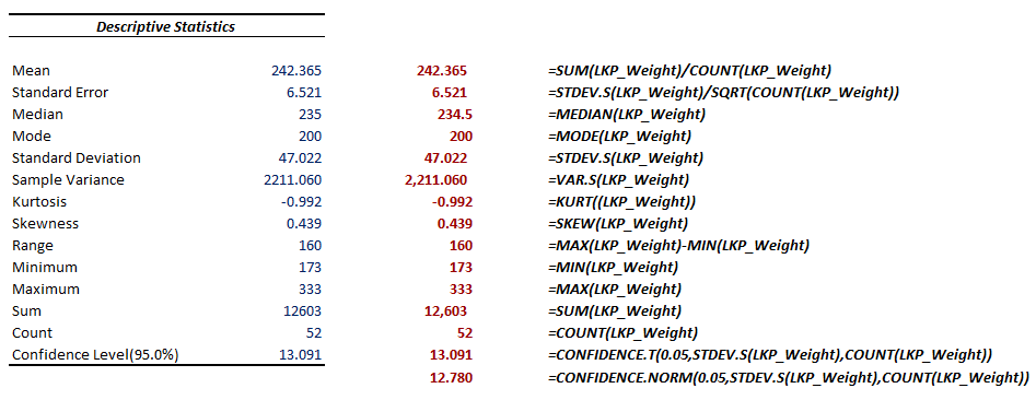
Mean – Is the mathematical average (or simply an average) of our data range. In our case, the average weight of all active Bears players is an impressive 242 pounds. To emulate this calculation via a formula, we simply need to add up all of the individual weights of our players and divide that total by the number players. Given that I created a named range for the weight column [LKP_Weight] , such formula becomes: =SUM(LKP_Weight)/COUNTA(LKP_Weight)

Standard Error – Measures dispersion of weights across our team players. It quantifies variability of sample means from sample to sample. At 6.52 pounds it is a fairly small value suggesting that we have a fairly precise estimate for our true population mean – at 95% level of confidence. For our dataset it could be calculated as 242.4 ± (1.96 * 6.52), which means that we are 95% confident that the true population mean falls within the range from 229.62 to 255.18. Excel offers us a built in function for sample standard deviation [see later], as well as square root and count functions: =STDEV.S(LKP_Weight)/SQRT(COUNTA(LKP_Weight))

Median – Another form of an average, which finds the middle value of a dataset sorted in ascending order, which is particularly helpful when our data includes skewed results (i.e. outliers.) Note that a median player weight of 235 pounds is lower than our mean, pointing to the fact that we have some outliers in the higher-weight category. Half of the players weighs in under 235 pounds while the other half weighs over 235 pounds. =MEDIAN(LKP_Weight)

Mode – Shows the most common weight of our players, at 200 pounds it stands considerably lower than either mean or even median value. In fact, three out of 56 players report this weight. =MODE(LKP_Weight)

Standard Deviation – Computes the level of deviation of data points from the mean. A larger standard deviation, such as 47 in our sample indicates a considerable amount of variability across weights of our players. Luckily Excel offers a built function for standard deviation, se just need to specify whether we want to calculate it for the Sample [S] or Population [P], setting for the sample for our purposes. =STDEV.S(LKP_Weight)

Sample Variance – Assesses average squared deviation of individual weights from the sample mean weight. In other words, 2,211 sample variance is our standard deviation squared [47^2.] Similarly, to the Standard Deviation, Excel offers us a Sample Variance function [VAR.S] =VAR.S(LKP_Weight) Notice that mathematically this is the same as =STDEV.S(LKP_Weight)^2

Kurtosis – Estimates the shape of the distribution of our data. A negative kurtosis (aka platykurtic distribution), such as -1 in our sample indicates that our data is less peaked and has lighter tails compared to a normal distribution. In other words, it is flatter and more spread out around the mean. KURT Excel function can perform this calculation: =KURT(LKP_Weight) Please see the figure below for further illustration.

Skewness – Measures the asymmetry of the distribution, particularly in terms of whether the tail on one side of the distribution is longer or fatter than the other side. The positive skewness of 0.44 can be interpreted as our that data distribution being skewed to the right, meaning that there may be some data points with higher values than the majority (please recall our discussion on Mean vs. Median), which is causing the tail on the right side of the distribution to be longer. SKEW is the Excel function for this metric =SKEW(LKP_Weight)

Range – Demonstrates the spread of the data, in our case variance between the heaviest player’s weight and the one putting the least pressure on the scales is 160 pounds [333 – 173]. =MAX(LKP_Weight)-MIN(LKP_Weight)

Minimum – Darnell Mooney, weighing in at “only” 173 pounds shows the smallest weight on the team. =MIN(LKP_Weight)

Maximum – Larry Borom and Darnell Wright are the heavysets of The Bears coming in at a massive 333 pounds. =MAX(LKP_Weight)

Sum – Cumulative weight of all players combined comes to whopping 6.3 US Tons. =SUM(LKP_Weight)

Count – Number of players on the team is 52. =COUNTA(LKP_Weight)

Confidence Level – Indicates a range of within which the true population mean would fall. We are 95% confident that population mean would fall within +-13 pounds of our sample mean weight of 242 pounds. In other words that range becomes 229 pounds through 255 pounds.

BONUS Exercises

Fortunately Summary Statistics is not the only tool within the mighty Data Analysis Toolpak. We can for example draw a histogram of the weight distribution in our sample. Data –> Data Analysis –> Histogram. Let’s specify the same range of cells representing weight of the team players, while also choosing three bins of weights: 200, 250, 300 [$N$5:$N$7] Effectively Excel would count number of players weighing in at or below 200 pounds, between 200 and 250 pounds, between 250 and 300 pounds, AND a fourth category calculated on the fly – for players falling above 300 pounds.

We can utilize dynamic array capabilities of modern Excel and utilize the FREQUENCY function to replicate histogram calculations formulaically:

If you are looking for more practice, perhaps you’d like to perform similar analysis on the height of the players now?

To close out this discussion, we can use either Data Analysis Toolpak OR Excel Functions to calculate both correlation [CORREL function] and covariance [COVAR function] of the weights in the roster of Bears players.

Correlation measures the strength and direction of a linear relationship between two variables. Plugging the data for the weight AND height of our players, we find positive correlation of 0.69, which is quite strong and positive, suggesting a substantial linear relationship between the height and the weight of our players. This means that as height increases, the weight tends to increase as well, and as height decreases, the weight tends to decrease.

Feel free to download the working version of my solution file.

Did you find this post useful? What is going to be the next dataset that you will be analyzing?