I personally don’t know why it took this long for Microsoft Excel team to create XLOOKUP function. The fact that VLOOKUP is considered to be one of Excel’s most widely used functions reflects a strong demand in string look up tabulations. Surely, a multitude of VLOOKUP‘s limitations can be overcome with patience, helper columns, INDEX/MATCH, CHOOSE, OFFSET and other constructs. Yet, why would we use any workarounds, when we would rather utilize a more powerful function with multitude of applications? Meet, much anticipated XLOOKUP function, which was officially released to Office 365 subscribers in early February of this year. It offers a really long list of additional benefits; in today’s tutorial we will review 11 scenarios that take full advantage of the following XLOOKUP features:

• LEFT lookup
• Horizontal lookup
• Multi-cell/array retrieval
• Match based on wildcard conditions
• Combination of Vertical AND Horizontal lookups
• Lookup based on multiple criteria
• Lookup in reverse order
• Lookup for maximum/minimum values
• Built-in Error Handling
• Exact match by default
• Flexible approximate match

To get started, let’s get acquainted with XLOOKUP‘s syntax. This function returns an item or items corresponding to the first exact match it finds based on your search. In addition to exact match, it can also retrieve the closest match. You might think that so far this sounds a lot like VLOOKUP functionality. Yet, we can also return values to the LEFT of our search arguments; we can retrieve more than one item at a time; error handling is built-in; we can specify the rank or the type of closest match; and finally, we can order our search results:

=XLOOKUP(lookup_value, lookup_array, return_array, [if_not_found], [match_mode], [search_mode]) 

lookup_value – {required field} – value you’re trying to look up/match.
lookup_array – {required field} – array that contains values you are searching for.
return_value – {required field} – array to be returned as a result of this search.
[if_not_found] – {optional field} – by default if a match is not found, this function will raise #N/A error; optionally we can substitute such error with a more relevant message or a value.
[match_mode] – {optional field} – specify the match type on how to match lookup_value against values in lookup_array.
0 – Exact match. If none found, #N/A would be returned by default.
-1 – Exact match. If none found, retrieve the next smaller item.
1 – Exact match. If none found, retrieve the next larger item.
2 – A wildcard match where:
? – searches for any single character
* – looks for any number of characters after the asterisk.
[search_mode] – {optional field} – provide the search mode to use:
1 – Default: perform a search starting at the first item.
-1 – Perform a reverse search starting at the last item.
2 – Binary search that relies on lookup_array being sorted in ascending order. [If not sorted, invalid results will be returned.]
-2 – Binary search that relies on lookup_array being sorted in descending order. [If not sorted, invalid results will be returned.]

Examples:

Example 1 – looking up matched value to the right of the search term.

Let’s suppose we had a list of largest cities in Missouri and needed find out population of Kansas City:

If we place our lookup value into cell F6 we would write our formula by specifying parameters used:

lookup_value : F6 – name of the city to lookup [Kansas City]
lookup_array: $B$4:$B$10 – Range of cells B4:B10 lists the names of the cities we want to search in to retrieve our city of interest: Kansas City. Using absolute cell reference is not required in our situation, yet is actually a good practice if we intend to copy our formula to other cells.
return_array: $C$4:$C$10 – this array houses population numbers for the cities in the previous range, and this is where the value of our interest will come from.
Putting it all together we would have:

=XLOOKUP(F6,$B$4:$B$10,$C$4:$C$10)

In case we wanted to handle errors, we could add optional [If_not_found] clause to our parameters and print “Not Found” message whenever there is no match found. This solution is a bit more elegant than adding a separate IFERROR function to our formula:

=XLOOKUP(F6,$B$4:$B$10,$C$4:$C$10,”Not Found”)

This is what our solution would look like:

Example 2 – looking up matched value to the left of the search term.

In the previous example we didn’t accomplish anything that couldn’t have been done using the standard VLOOKUP function. Imagine we had a list of cities in Kansas City metro area spanning two states. If we wanted to find out which state Overland Park is located in and we placed our search term into cell G6, our formula would look something like below:

=XLOOKUP(G6,$C$4:$C$15,$B$4:$B$15)

WHERE:
lookup_value : G6 – name of the city to lookup [Overland Park]
lookup_array: $C$4:$C$15 – Range of cells C4:C15 lists the names of the cities we want to search in to retrieve our city of interest: Overland Park. 
return_array: $B$4:$B$15 – this array includes state names corresponding to cities in the previous range.

This is the first example of XLOOKUP‘s magic gracefully overcoming numerous limitations of VLOOKUP function.

Example 3 – looking up matched value based on multiple criteria.

3A. Multi-criteria lookup from one cell.

Let’s say we didn’t know which state Super Bowl LIV winners called home and tried to look up population of Kansas City, KS , below formula would do the trick, assuming we placed our search criterion in cell G6 (note that ‘Kansas CityKS‘ as one word is the only valid search term here as either or ‘Kansas City KS‘, or ‘Kansas City, KS’ will not find a valid exact match.)

=XLOOKUP(G6,$C$4:$C$15&$B$4:$B$15,$D$4:$D$15)

Let’s dive in:
lookup_value and return_array should make sense by now, yet lookup_array is of particular interest here.
lookup_array: $C$4:$C$15&$B$4:$B$15  – If you recall, range of cells C4:C15 lists the names of the cities we want to search in to match the city search, the ampersand sign [&] helps us join search criteria and add another array B4:B15 to search for the state of interest. As a result we are combining two disparate search arrays in one formula. Please note that using one range of B4:C15 would not work here.to retrieve our city of interest: Overland Park. 

Feel free to take a minute to take in the power of XLOOKUP…

3B. Multi-criteria lookup from one cell – approximate match.

In the above illustration we already discussed that ‘Kansas City KS‘ search term would yield an error as we would not be able to find exact match. At the same time, we also recall that this powerful function does allow a couple of different ways to handle approximate matches, should that exact match not be found. In fact we can use 1 as an input for the optional [Match_mode] parameter to instruct Excel to retrieve the next larger item in the absence of exact match:

=XLOOKUP(G6,$C$4:$C$15&$B$4:$B$15,$D$4:$D$15,,1)

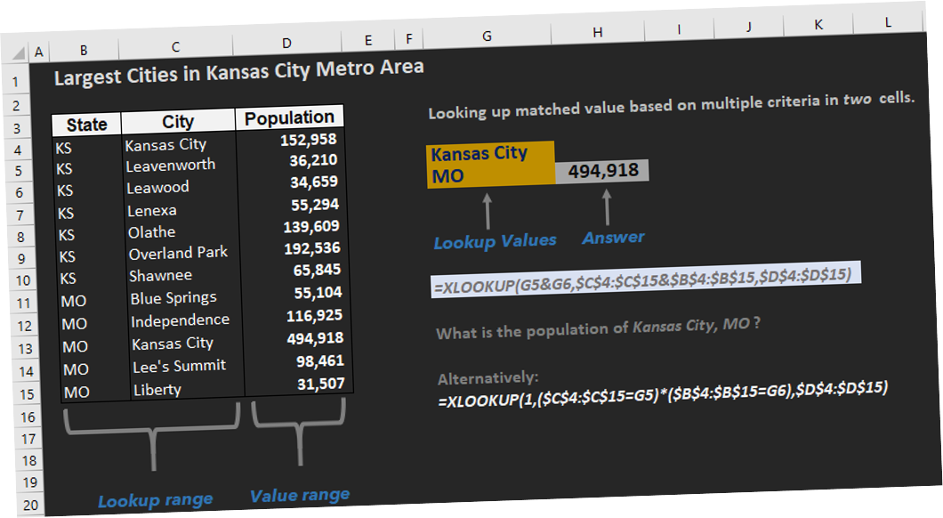
3C. Multi-criteria lookup from two cells.

Let’s test the flexibility of this function even further, shall we? If cell G5 contained Kansas City string, while G6 included KS search term, we could concatenate them into one combined criterion within [Lookup_value]: G5&G6 like so:   

=XLOOKUP(G5&G6,$C$4:$C$15&$B$4:$B$15,$D$4:$D$15)

Alternative solution allows us to search one criterion per respective search array at a time. Knowing that, would you be able to decipher the below formula that yields the same result?

=XLOOKUP(1,($C$4:$C$15=G5)*($B$4:$B$15=G6),$D$4:$D$15)

Example 4 – looking up matched value based on exact match OR lower.

Similarly to the above example, what if we wanted to look up the name of the city with 100,000 residents, or lower if the search does not produce exact match. Our [Match_mode] need to be set to -1. Since our list does not contain exact match (no cities with exactly 100,000 residents), below formula returns ‘Lee’s Summit‘:

=XLOOKUP(G6,$D$4:$D$15,$C$4:$C$15,,-1)

Example 5 – retrieving matched value based on a wildcard condition.

Let’s suppose we are not sure how to spell how to spell our search term. Wildcard search can help in this case. Let’s say we want to look up population of Olathe, KS ; yet we’re not sure how to spell full name of this town and only know first two letters. With cell G6 containing string ‘Ol‘, our [Lookup_value] would become G6&”*”. We also need to help Excel identify this search as a wildcard search by setting [Match_mode] to 2, like so:

=XLOOKUP(G6&”*”,$C$4:$C$15,$D$4:$D$15,,2)

Example 6 – looking up matches based on the lowest or largest value.

Here is yet another search you couldn’t do with a simple VLOOKUP. Wrapping MIN/MAX functions inside our [Lookup_value] parameter allows us to quickly figure out our data boundaries. To determine that Liberty (population of 31,507) is the smallest city on our list, we can use the formula below:

=XLOOKUP(MIN($D$4:$D$15),$D$4:$D$15,$C$4:$C$15,,1)

While the below alternative won’t work for the Maximum condition, we can rewrite our formula without using MIN function by providing unrealistically low number and setting [Match_mode] to 1:

=XLOOKUP(0,$D$4:$D$15,$C$4:$C$15,,1)

Example 7 – looking up a match based on the first/last value in the list.

What if you needed to simply retrieve the first value in the list? No worries, XLOOKUP can handle this task with ease. We first need to pass a wildcard to our [Lookup_value] parameter, then set [Match_mode] to wildcard search: 2, and close off by specifying our [Search_mode] to retrieve the first value of 1 in our list to return Kansas City.

=XLOOKUP(“*”,$C$4:$C$15,$C$4:$C$15,,2,1)

Example 8 – looking up a value based on the first/last match in the list.

Building upon the previous example, we can do something that was previously not possible with VLOOKUP function – take control of the order of our retrieved values. Surely, in most cases you are looking to retrieve the first match from the list, yet there will be some use cases when the last match is needed. If you recall, we have two Kansas Cities in our list, Kansas City, KS with population of 152,958 and Kansas City, MO with population of 494,918. Working with values for the [Search_mode] parameter we just introduced, we can set it to 1 for the first match and -1 for the last match. First formula below will yield 152,958 as Kansas City, KS is the first exact match found, while the second formula will search in reverse order and return 494,918:

=XLOOKUP(G6,$C$4:$C$15,$D$4:$D$15,,,1)

=XLOOKUP(G6,$C$4:$C$15,$D$4:$D$15,,,-1)

Example 9 – looking up matched values from multiple cells.

Yes, you read it correctly, in this example we will retrieve values, as in more than one value from our search. If you are still not yet convinced in the power of XLOOKUP function, perhaps seeing “Spilled” formula feature at it’s best might do the trick. Let’s suppose we added Rank field to our dataset, could we retrieve State, City, and Population values all from one formula? The answer is, absolutely:

When it comes to [Return_array] parameter we simply need to specify all three columns to be returned B4:D15, like so:

=XLOOKUP(G6,$E$4:$E$15,$B$4:$D$15)

We then need to accept default settings for Excel’s Spilled Formula dialog box below and viola, we are done, Excel automatically retrieves multiple columns of data for us.

Example 10 – looking up matched value below the searched term [a.k.a. HLOOKUP).

We already mentioned that XLOOKUP is in fact rather flexible function, not only will it effectively replace and augment VLOOKUP‘s functionality, it will also be able to replace horizontal lookup function – HLOOKUP as well. All we need to do is to pass rows instead of columns to our [Lookup_array] and [Return_array] parameters. Hopefully you will be able to follow example below which helps us retrieve population-based rank of city of interest, where city name is contained in cell K6:

=XLOOKUP(K6,$C$3:$I$3,$C$5:$I$5)

Example 11 – Looking matched values from both: rows and columns (VLOOKUP + HLOOKUP)

Let’s wrap-up this post with an example showing combined impact of looking up from both: rows and columns. By now this illustration should be self-explanatory:

In one of our next posts we will revisit and solve these problems using Google Sheets‘ answer (or more precisely a preemptive strike) to XLOOKUP – QUERY function – Stay Tuned!

If you are interested in Excel workbook companion for this tutorial, feel free to download it from our site.

Have you had a chance to use XLOOKUP function yet? What is your favorite feature so far?