During these uncertain times, how can you make sense of the data tsunami being presented on the state of pandemic in US? For the last couple of months, many Americans found themselves checking the spread of COVID-19 cases on a daily basis. As most of US states went into shelter-in-place mode, resources like Johns Hopkins and 91-DIVOC became a daily refuge for those seeking to stay informed. In today’s post, we will work on creating our own version of a web-based, interactive and visually appealing COVID-19 dashboard using Google DataStudio. Doing so we will gain a better understanding of the data used, decide on the type of data we deem most relevant, and maintain control over the best ways to visualize such data to help our audience make most sense of it. In the process of building this data viz, we will utilize various objects and features of the mighty GDS application: Google Sheets connector, Calculated fields, Scorecard, Table, Geo Map, Line and Combo charts, Date range, Filter controls and recently released optional metrics – are some but not all features we will cover.

Data Selection and Initial Preparation

The first step in any data visualization project is determining the type of data we need to chart. In our case, it would be helpful to show the spread of the virus by state, as well as potential reversal in its growth rate, if applicable. New York Times seemed to be a reliable enough of a data source for our project – luckily they make this data available on their GitHub repository. In fact, we have an option of consuming this data at the state vs. county level. For simplicity’s sake, we will use the state-level of granularity in our report. Looking at NYT’s file, they seem to only show cumulative COVID cases and deaths. While cumulative pandemic charts seem to dominate the COVID-19 reporting space (i.e. Johns Hopkins), I would argue that other portals that also offer growth rates (91-DIVOC et al.) are better suited for monitoring spread of this disease.

In the case of cumulative reporting, we will always (with the exception of data issues identified later) have next day’s data point being equal or greater than the last day’s; as such, looking at the resulting graph, it would be fairly difficult to identify the level of gradual growth. Alternatively, looking at the new cases only, or better yet, plotting case growth could help us assess if the infection is in decline.

We also need to acknowledge the fact that confirmed cases data does not offer like for like comparison across US states, as different states had differing level of preparedness when it comes to testing its residents. At the same time, it would be irresponsible to ignore state population when it comes to gauging the spread of the disease and especially COVID-related deaths. (Arguably more accurate measure of potential infection rate, yet still not accurate due to varying and often subjective rules when it comes to assigning cause of death by state, municipality, etc.) In order to look at the population-based metric, we will also bring US Census data to the mix.

Using NYT‘s data, we will calculate new cases and deaths by state/date combination. In the spirit of further developing our data, we can also calculate Day Over Day Growth rate and 7-Day Moving Average Growth. As a final data preparation step, we would need to blend COVID data with state population to estimate daily Cases per Capita and Deaths per Capita metrics.

Naturally, our job wouldn’t be complete without some data cleansing. According to this source, cumulative total of COVID-19 cases in Georgia changed by -158 when this reporting went from 12,261 on 4/11 to 12,103 on 4/12. Idaho experienced a similar fate, when its total dissipated by 2 cases from a reported number of 2,061 on 5/2 to 2,059 on 5/3. In these critical times, when we need “data, evidence and science”, these data quality issues are particularly bothersome. World Health Organization reported US having -99 (!) new cases of COVID-19 on Sunday. Apparently, they switched reporting methodology to align with CDC, yet didn’t think of making retroactive adjustments. To account for these irregularities and to minimize the impact of misleading growth rates, I replaced all calculations yielding negative new cases with the value of 1. This means that adding up New Cases will not match Cumulative Total, but I believe this would be a lesser of two evils we are dealing with here. To normalize our charting scale, I applied a 200% Day over Day growth ceiling to all readouts exceeding this value. While at it, I also excluded all US Territories from this worksheet.

You can access resulting Google Sheets workbook for the next steps in our process. Make sure to save it to your Google Drive.

Creating a new report

Unlike many other data visualization applications, DataStudio does not require software installation, nor does Google charge any fees for using this program. We simply need to log in to our Google account and navigate to DataStudio’s home page (preferably using Chrome browser) to start using this powerful tool. Click on the large plus sign at the top of the left panel or the first selection on the main menu to start a new report.

Establishing connection to the data source

Before we even have a chance to name our report, we are asked to connect to the data source of interest. If we have already used a data source for another visualization and simply need to tap into it again, we would click on the My data sources tab to pick from the sources available. Otherwise we have to create a new data source by selecting from one of the 17 data connectors available for DataStudio integration. Luckily Google Sheets is one of the connectors available, let’s click on it.

We would then navigate to the workbook containing our data and select actual worksheet that houses it. As you might recall by now, our file is called ‘COVID-19_StateDate‘ and worksheet is named ‘StateData‘. Once you make this selection, keep all other defaults and click on ‘Add’ to continue and then confirm your intent to add this data by clicking on ‘Add To Report’ button.

Google then presents us a with a default view of the report. Before proceeding any further let’s ensure that our data source is using correct data types for our data. Selecting ‘Resource’ menu and ‘Manage added data sources’ sub-menu gets us to the below view, where in we need to click on ‘Edit’ to start our exploration.

While all other data fields seem to meet our criteria (more on this later), ‘State’ one needs to be adjusted from using Text data type to a Geo data, Region to be more precise. Once selected, follow ‘Done’, ‘Continue’ and ‘Close’ button sequence.

Report Formatting and Layout Options

We are now done with the most tedious part of our job – dealing with the data and ready to start working on a more creative and fun portion of it – actual data visualization.

At this time we are ready to name our report, select appropriate style and size for our dashboard. To rename current title simply overwrite file’s name found in the top left corner of the page with the one you like – I will call this dash ‘COVID-19 Cases By State’. Let’s then delete an unwanted data table DataStudio created for us by default by selecting that object and pushing Delete key.

When it comes to reporting themes, DataStudio offers more than a dozen options; let’s navigate to the one called ‘Edge‘ on the right panel of our window and select it as our theme. Finally, let’s resize our canvas size by either changing tab selection from ‘Theme’ to ‘Layout’ – selection applies to all pages on this report or right-clicking on report and following ‘Current Page Settings’ to make adjustments for the selected page only. Selecting ‘Page’ menu – ‘Current Page Settings’ would do the trick as well. I will set a custom canvas size 1,600 pixels wide and 800 pixels tall. Our report is starting to take shape:

Anyone using Google Sheets product will find DataStudio’s interface and functionality very familiar.

*File menu allows us to use different options to share our report (much like the Sheets feature with the same name), make a copy of the existing report, create a new report, and more.

*Edit menu will let us perform typical functions associated with such menu: Copy, Paste, Delete, Undo, etc.

*View menu options might appear to be fairly unexpected at a first glance, but certainly start making more sense over time. If your theme does not remove default grid options, you can control report’s grid using commands found here. Should you want to refresh your report based on most recent update in your data source you can also ‘Refresh data’ (?!) from this menu.

*We can add new pages to the report, rename, copy/duplicate existing pages and navigate through the report using the Page menu.

*When you have multiple pages in your file, you can control them (including their filter options) through the Arrange menu.

*We’ve already utilized ‘Manage added data source’ function found under the Resources menu, you can also manage and control other report functions: filters, blended data, parameters, and others.

*Help will do what you would expect from this menu, and interestingly enough it also lets you get Google engineers’ attention through a request for a feature you’d like to be added to the program.

*We skipped through the most interesting menu – Insert which enables us to actually add various elements: charts, images, text, date and filter controls, as well as shapes to our report.

Many of these commonly used objects can also be invoked by clicking on the corresponding icon found on program’s toolbar. Upon clicking on ‘Add a chart’ button we are presented with various chart objects we can utilize in our report: data and pivot tables, scorecard, line/bar/pie/area/scatter/bullet graphs, Geo and Tree maps:

Working with Non-Chart Objects

We are now ready to create our dashboard. One of my favorite features of DataStudio is full control of the canvas – we can place our objects anywhere we like and we can easily resize them to fit our needs.

To start we will add a title label to our report by clicking on the Text box object also found under Insert – Text menu. Let’s place this object in the upper left corner of our page, I will call it ‘US COVID-19 Cases By State‘. Let’s then adjust font settings – make it bold, switch default font to Roboto and change font’s size to 20. As a final touch, Google does not seem to recognize word ‘COVID’ let’s add it to program’s dictionary using right-click menu option.

It might be helpful for our audience if we also specified last reporting date, which happens to be 5/9/20 retrieved on 5/10/20 at the time of this writing. To cite our sources we will utilize another text box and place it at the bottom of our page. Right underneath Left justification button within Text Properties panel we can find Insert link button that lets us add a hyperlink to our text. Going through the hyperlink wizard, we can provide the text to display, share actual URL for our link, and ensure that link would open in a new browser tab:

GDS makes it easy to add images to our dashboard, at work you probably would incorporate company’s logo on your page. For our purposes let’s add a slightly modified attribution-free image depicting Corona Virus by clicking on the Image button immediately to the left of the Text box (also found in Insert – Image menu.) We have two options now: upload from our local drive or provide image URL. We will place this control in the top right corner of our canvass.

Next on the list is Date range control/filter which adds a layer of interactivity to our report. To draw audience attention to this control let’s go ahead and change background color of this date filter control, while also preserving consistent font typeface. We would need to utilize contextual Date range Properties panel found to the right of our canvass:

We also have a few options to manage actual date range, given our dataset, let’s settle for the fixed calendar starting on 3/8/20 (most states hadn’t started reporting confirmed COVID cases before then, and the ones that did: WA, CA, NY had less than 200 cases each) through 5/9/20 (last reporting date available):

Next control is technically considered a type of chart, yet in my book it’s a metric readout that DataStudio refers to as Scorecard :It can be found by either selecting Insert menu and going to Scorecard or finding this control via Add a Chart button on the toolbar. Using the Data tab via Scorecard panel we can set its metric to New Cases aggregated as SUM. This would allow us to keep a running total of all cases confirmed during the time period specified. Note that Date Range dimension is set to our Date [calendar] control. We can only use no more than one metric with this control at a time (optional metric selection is also available here), and there no non-date dimensions allowed:

When it comes to the Style tab let’s ensure that our metric is using compact numbers (Millions, Thousands, etc), change our font to Roboto, size 24. And finally remove all borders and make this control completely transparent. Note that as part of its continuous improvement and roll-out of enhancement GDS recently added conditional formatting functionality to its list:

To visualize separate this scorecard from other controls, let’s enclose it within two line shapes (Insert – Line.)

We will repeat these steps to also depict number of new deaths.

A common theme within many COVID-related visualizations is that with the exception of some of the better ones (already mentioned 91-DIVOC and the like) is that they don’t typically normalize their datasets based on population size. Californians exceed the number of Wyomingites by the factor of almost 70(!), it might make sense to consider this fact when it comes to understanding potential infection rates [Yes, I do understand that most of COVID carriers are probably not tested, but these confirmed case numbers is the best signal we have to measure disease spread outside of using a more morbid metric – number of deaths.]

While our dataset already includes number of cases and deaths per capita, demographers often use Per 100,000 measures for better readability. Multiplying our per capita values by 100,00 would yield this desired outcome. This can be accomplished through using a calculated field feature. Let’s navigate to the Resources tab and choose Manage added data sources option to edit our data source. We would then click on ‘Add A Field’ button to open calculated field wizard.

We can remove likely unnecessary decimal points by using the ROUND function in conjunction with our multiplication for the Cases Per 100K field :

Click Save, then DONE to save your changes. Repeat for Deaths Per 100K calculation. Let’s then create corresponding scorecards for these measures using MAX aggregation – effectively corresponding to the last date used in our date range. Note that this would limit our calculations to be valid at state level only and prevent us from using country-wide metrics. Other notable metrics to show could Maximum number of new cases per day (make sure you rename this metrics as needed), Median number of cases in our range and finally last day’s 7-day Moving Average growth rate. Earlier in this exercise we chose to not change any data types in our source data, luckily we can reformat our data type for the specific control only – let’s make sure that we change our number format to Percent:

When done, we could choose to have metrics similar to the below:

Working with a Geo Map

Since we have State as one of the fields in our data source AND because we were able to reformat it as Geo data type we can now build an interactive map of US states. Let’s plan on placing this chart in the upper left quadrant of our planned layout. When it comes to conditional formatting, we can color this map based on any metric available, in our case we will use ‘Deaths Per 100K‘. Going to Insert menu and selecting Geo Map option will get us started here.

GDS will automatically put Date into the ‘Date Range Dimension’ section, recognize State a ‘Geo Dimension’, our job is to simply specify Deaths Per 100K as a ‘metric’. In an unlikely chance of ‘zoom area’ extending beyond US borders it would be helpful to make the appropriate change. Final step within the ‘Data’ tab would be checking the Apply filter box found under the ‘Interactions’ section. This one, yet powerful mouse click will magically add interactive capabilities to our map control, letting us filter the rest of the report based on the State selection:

Moving to the ‘STYLE’ tab of our panel, we would work with the ‘Geo Map Chart’ color options to conditionally format Max/Mid/Min color values:

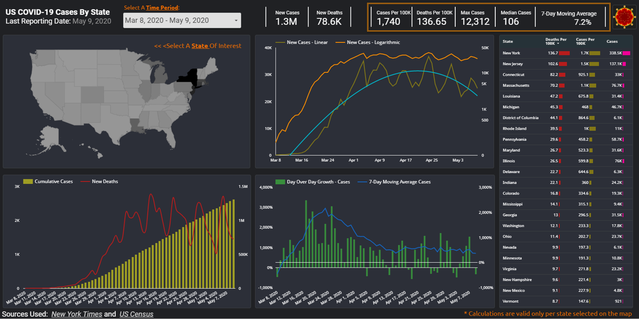
Resulting Map quickly shows population-adjusted COVID deaths data and allows us to select a state of interest to focus our analysis efforts. It also looks fairly presentable now:

Plotting Linear vs. Logarithmic Values on a Time Series Graph

One of the great ideas I picked up from the 91-DIVOC site is plotting values on a logarithmic scale. This could be helpful since during the exponential growth (i.e. initial spread of COVID) it would be easier to spot trends using log scale. Utilizing dual axis feature of a time series graph we can have the best of both worlds: plot New Cases values on linear and log scales. While at it we will add a Trend line to our chart.

Metrics section allows us to place more than one measure on our chart. In this example we will use ‘New Cases’ twice. ‘STYLE’ tab lets us choose between Line vs. Bars chart type for our time series visualization, we can specify color of preference, line weight, and dual axis Ys by switching between Left vs. Right axes. Trendline feature allows for Linear Exponential, and Polynomial depiction of trends. You might want to consider making the below choices in this chart.

After checking the Log scale box on the appropriate axis our time series graph has all of the pertinent charts to aid us in better assessing trends associated with the spread of COVID:

Showing Line and Bar Charts on a Dual Axis Time Series Graph

A more traditional use of a dual axis graph would be using disparate scales and possibly choosing different chart types. This is precisely what we will do next. One of the axes would show number of Cumulative Cases on a bar chart, while the other axis will plot number of New Deaths over time via a line chart. A welcome addition to GDS was introduction of optional metrics. To help our users better interact with our dashboard we are now able to let them specify a metric of interest. For example, we can add Cumulative Deaths to the appropriate section of the chart’s DATA tab:

Assuming we enabled chart’s header to ‘Show on hover’ [STYLE tab], users would be able to pick and choose from metrics to utilize in their custom graph:

This easy to use feature could empower our audience to become analysts in their own right. Looking at the resulting graph without optional metric, we can compare two different trends over time:

Tracking New Case Growth Rates

Next chart is definitely one of the most important on our dashboard. In fact it attempts to help us make sense of the data at hand – at which time period do we experience new case growth or relative decline? Luckily as described in the Data preparation section we have just the right metrics for this task. I will trust in your abilities to find the right way to chart Day Over Day growth rate in New Cases, as well as 7-Day Moving Average of New Case growth. Looking at the hardest-hit state, things appear to be looking up for New Yorkers, they are far away from April 4th high of 12,312 New Cases and the growth rate is trending near or in the negative territory:

Using Data Tables with Bars

Providing raw data for user consumption is a common practice to help users gain access to information that’s not easy to summarize on a chart due to the sheer volume of records present and disparate units of measurement used. Luckily we can incorporate DataStudio’s Table object, or better yet, Table with bars [combination of actual data AND visual representation of said data points] to accomplish this task. Those of us coming to DataStudio from Google Sheet or dare I say MS Excel will find this functionality very familiar. STYLE tab would allow you customize the look and feel of your data. Below table shows Deaths Per 100K, Cases Per 100K and New Cases metric aggregated at the State level for the time period specified:

Sharing Our Work

Congratulations, our work is now done, one last step is sharing our data viz with folks who would be consumers of our report. Google provides great control in terms of who we want to provide access to and the type of access granted. Similarly to other Google products, DataStudio allows us to let everyone on the Web access our work, restrict access to those with the link (route we are taking here), anyone within our organization, anyone within our organization with a link, or rather limiting it to the specific few we call out by sharing their email address information. To find these options follow the File menu, select Share, and then click on ‘Get Shareable Link‘:

To view visualization we just created, please feel free to follow this link.

Which other metrics would you consider adding to this dashboard? Are there any other data visualizations you would incorporate in this dashboard?